Mode sets and transverse quadrature#
A multimode calculation has two spatial choices: which modes to retain, and where to evaluate the nonlinear response across their shared cross-section. Increasing the number of modes and increasing the quadrature resolution address different errors. The RDW lesson shows how to interpret the resulting modal energies.
The transverse quadrature#
The multimode transform integrates over the cross-section with one fixed rule, chosen once per problem, never an adaptive one. The argument is not economy. The Kerr polarisation is cubic in the field, so its projection is a quartic in the transverse profiles; those are Bessel functions of \(r/a\), analytic, and a Gauss rule of modest order integrates a quartic of them to rounding. Measured against a 2048-node reference, the quartic overlap tensor of four \(\mathrm{HE}_{1m}\) modes is converged to \(2\times10^{-14}\) at \(n_r = 32\) — the reference’s own rounding, not the rule’s.
Radially, \(n_r\) Gauss–Legendre nodes on \(\xi = r/a \in (0,1)\), with the Jacobian and
the azimuthal \(2\pi\) folded into the weights, \(w_i = 2\pi a^2\xi_i w^{\rm GL}_i/2\). The
nodes are strictly interior, so the wall is never sampled. With radial_rule="gauss_kronrod" (the
capillary default) the count is rounded up to \(2n+1\) and the rule becomes the Kronrod extension of the \(n\)-point Gauss rule, whose
Gauss subset is an embedded coarse rule: the difference of the two projections is an
error estimate that costs nothing, because the two rules share every node the coarse one
has. solprop computes that extension with Laurie’s algorithm rather than shipping a table,
so any order is available, and checks it node by node against the Julia package
QuadGK.jl’s implementation of the same algorithm.
In the field scale, for one Marcatili HE₁₁ mode in a uniform gas, the radial
projection is an integral over \(\eta = J_0(u_{01}r/a)\), and radial_rule="field_scale"
and "field_scale_radau" are the Gauss and Gauss–Radau rules for it: exact for the
linear and Kerr source from two (Radau: three) nodes, the Radau rule with one node on the
axis, and the one-node member the effective-area model. They carry radial area weights,
have no embedded coarse rule, and refuse any other mode set. When to use them, with the
evidence, is in radial nodes for expensive responses.
Azimuthally, \(n_\theta\) equispaced nodes offset by half a step — the periodic
trapezoid rule, which is a Gauss rule on the circle and is exact for trigonometric
polynomials of degree at most \(n_\theta - 1\). A quartic product of modes with azimuthal
order up to \(h\) reaches degree \(4h\), so
transverse_quadrature() warns below
\(n_\theta = 4h + 1\); the default 16 covers \(h \le 3\).
The offset is not cosmetic. On-grid nodes at \(0, \pi/2, \pi, 3\pi/2\) annihilate products such as \(E_xE_y\) for a superposition of hybrid modes, so two successive levels of an adaptive rule both return zero, the level-to-level error estimate is zero, and the integrator declares convergence on a wrong value. The fixed offset rule cannot be fooled that way, and has no convergence decision in it to fool.
What the tensor is worth checking against#
The rule’s job is one number per pair of modes, and for a set of \(\mathrm{HE}_{1m}\) modes that number has a closed form worth stating, because it is the whole of the intermodal Kerr coupling at leading order. A field that is the fundamental alone drives a polarisation \(\propto \hat e_1(r)^3\), which factorises: whatever the pulse, the response, the shock term or the third harmonic, the drive it projects into mode \(p\) is that of mode 1 times
For the first four modes that is \(1\), \(0.4785423\), \(0.0221346\) and \(-0.0023723\) — geometry, with no gas, no wavelength and no normalisation constant in it. The fourth is negative because \(J_0(u_4r/a)\) changes sign three times inside the bore. The fundamental’s own entry has a closed form too,
which is the identity that makes a one-mode multimode run and a mode-averaged one agree. The transform’s overlap tensor reproduces these ratios to better than \(10^{-11}\), so when the higher modes of a multimode \(\mathrm{HE}_{1m}\) run look suspicious, the intermodal Kerr coupling is not the place to look.
Tapers cost two scalars#
For a scale-invariant mode the profile depends on \(r\) only through \(r/a\) and \(N \propto a^2\), so at nodes placed at \(r = a\xi\) the normalised field is exactly proportional to \(1/a\) and the weights to \(a^2\). Moving along a taper therefore rescales the matrices exactly:
which is rescaled(), and their product — the
thing the transform actually applies — does not move at all.
Mode sets#
ModeCollection is an ordered set of modes sharing one
cross-section, validated once, because the mode axis of the kernel state is positional and
one transform matrix serves the whole set. It reports the highest azimuthal order and
whether the azimuthal coordinate has to be resolved, and it is a Sequence[Mode], so the
quadrature and the mode matrices take it directly.
For a vector run, with_polarisations()
expands a spatial set into the polarisation-resolved one: each hybrid mode is followed by
its partner, the same mode turned by \(\pi/(2n)\), which turns the pattern a further
quarter turn from \(x\) towards \(y\) and so exchanges the two Cartesian components: the
pair runs \(x\) then \(y\) for \(\mathrm{HE}_{1m}\). A transverse mode is carried once —
\(\mathrm{TE}_{0m}\) and \(\mathrm{TM}_{0m}\) are different modes, not two states of one.
orthonormality(), which a simulation runs
on every mode set it is given, integrates adaptively, deliberately not on the fixed
rule, so that the rule’s orthonormality is checked against something independent rather
than against itself. It integrates the whole matrix in one pass: adaptively in \(r\) (or
\(x\)) with scipy.integrate.quad_vec(), every mode evaluated once per point, and on
a rule in \(\theta\) (or \(y\)) doubled until no entry changes by more than \(10^{-12}\); it
refuses a set on which either coordinate does not converge, and takes seconds for 48
modes. overlap() is its entry for one pair. Step-index
channels of one fibre each bound the cladding at their own outer radius; their set is
integrated over the widest of those discs.
A capillary worked example#
The four lowest \(\mathrm{HE}_{1m}\) modes of a helium-filled capillary, evaluated directly from their mode objects: the transverse profiles a multimode run projects onto, and the loss each carries.
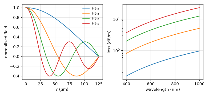
The four lowest HE_1m modes of a 125 um capillary filled with 1 bar of helium. Left, the transverse profiles: each is a Bessel function of r/a vanishing on the wall, and they are mutually orthogonal, which is what the quadrature rule has to reproduce. Right, the loss, which grows as the square of the Bessel zero u_1m and as the inverse cube of the radius – HE_14 leaks 24 times faster than HE_11.#
The zero-dispersion wavelength follows from the balance between the gas and the waveguide, and moves with pressure:
from solprop.modes import MarcatiliMode
from solprop.modes.base import zdw

mode = MarcatiliMode(125e-6, "He", 0.4, model="reduced")
zdw(mode)  # 3.767e-07 m
zdw() samples the sign of \(\beta_2\) at 512 frequencies across the
window and refines each change. Each change is then one of three things.
A zero, where the analytic group delay \(\beta_1\) has an extremum that the difference behind \(\beta_2\) resolves – its rise from the change grows quadratically over the difference’s stencil, on both sides – and is monotone from it for 1.5 % in frequency on either side, so that \(\beta_2\) keeps each sign that far.
A line, where \(\beta_1\) is not finite or not continuous: across the stencil it diverges, or drops to the evanescent floor, by more than a tenth of its value. A gas resonance in the vacuum ultraviolet gives the differenced \(\beta_2\) sign changes of this kind that are not zeros (krypton has sixteen between 100 and 124 nm at 15 bar): through the line’s pole, where the stencil reaches a line, and on the evanescent floor above one.
Fine structure, anything else: a change the stencil does not resolve, or one of the clustered zeros of a narrow feature that leaves \(\beta_1\) finite and continuous. Fused silica’s OH absorption bands are the common case: optmat’s silica (Franta’s model of a synthetic glass, OH bands included) flips the sign of \(\beta_2\) four times between 1.37 and 1.40 µm, through regimes 0.2-0.8 % wide, and again near 2.2 and 2.7 µm, while its group delay varies by \(10^{-4}\) and 5 % of its value. The inside of an antiresonant wall’s resonance can hold zeros closer than 1.5 % too; the zeros on its flanks, which bound the normal dispersion beside it, lie 2 % or more from the next in the fibres checked, and are zeros. Fine structure is passed over: it is neither a zero nor a line.
The search therefore resolves dispersion regimes 1.5 % wide and more, and its answer does not depend on the window, as long as the window holds the zero: a standard telecom fibre (NA 0.12, a 4.1 µm core radius) reports 1295.8 nm from a 1550 nm reference on a 100 nm to 3 µm window, on 0.7 to 2.5 µm and on 1 to 2 µm alike, past its 1.38 µm OH band. Its limits: two genuine zeros closer than 1.5 % (or a zero within 1.5 % of another sign change) are passed over, a zero and another sign change inside one sample interval restore the sign and are both missed, and a sample that is not finite brackets nothing.
The default window runs from 150 nm to 3 µm: above the vacuum-ultraviolet lines of the
noble gases (the longest, xenon’s, at 147 nm) and the absorption edge of fused silica,
below which a lossless solve takes silica as transparent and finds zeros with no
meaning. A deep-ultraviolet zero needs wavelength_limits set below it.
A window can still hold several zeros: two zero-dispersion wavelengths, or the gas’s own
zeros between two of its lines. Without near the call refuses them by name; with a
reference wavelength near (typically the pump) it returns the zero nearest it in
frequency among those no line separates from it, since light at the reference cannot
cross a line to reach the others:
krypton = MarcatiliMode(14e-6, "Kr", 15.0)
zdw(krypton, wavelength_limits=(100e-9, 3e-6))
# ModeError: beta2 has 3 zeros over 100-3000 nm, at 108.9, 119.9, 770.5 nm
zdw(krypton, wavelength_limits=(100e-9, 3e-6), near=800e-9)  # 7.705e-07 m
zdw(krypton)  # 7.705e-07 m: the default window starts above the lines
When the search finds no zero it raises
NoZeroDispersionError, rather than returning a missing value
that would propagate silently into later arithmetic: a mode with no zero-dispersion point
is a fact the caller has to see.